Statistical Analysis |  Tutorial Main Menu | Applying R to Political Science

Section 5: Statistical Analysis Part 2

ANOVAS in R

In Figure 5-1 we will define three separate groups with 7 separate observations per group. Then, we will use n and group to combine the groups into vectors.

n =rep(7, 3) and group =rep(1:3, n) are vectors.

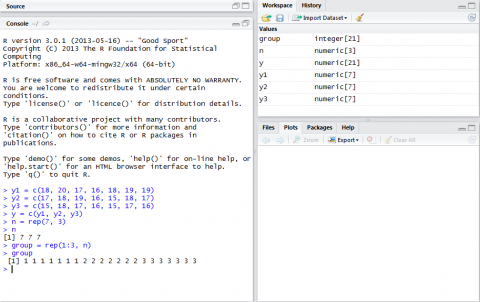
Figure 5-1

The tmp = tapply(y, group, stem) code is used to summarize the data by determining the decimal point locations. If the data contains all whole numbers then the output(on the right side of the vertical lines) would display zero's.

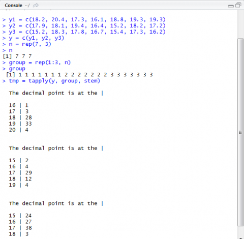
Figure 5-2

The tmpfn function is a temporary function to show the overall summary of the 3 groups of data by displaying the sum, mean, variance and the value of n.

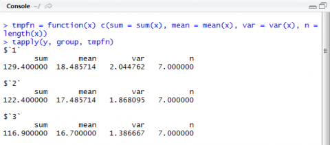
Figure 5-3

This is the summary of the information listed in Figure 5-4.

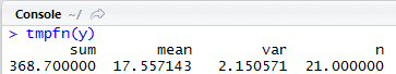
Figure 5-4

This code displays the ANOVA table into the R console.

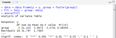
Figure 5-5

Frequency Distribution

We can create frequency distributions by manipulating a current dataset or by creating a new one.

Lets say we wanted to see how many students in a sample group liked blue. In this example we will be creating a boxplot to display the data. In Figure 5-6, we first import the dataset sample, which displays the ID, Color and Gender of the group.

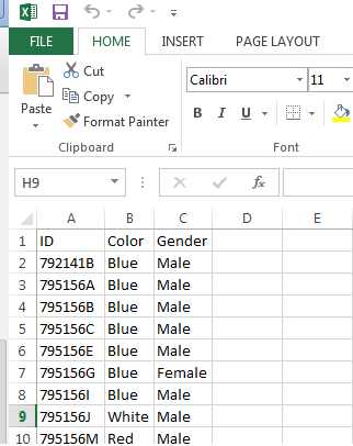
Figure 5-6

In the code, we defined the 4 colors that were given in the sample(blue, green, red and white). We also have yellow as a category to show what the graph looks like when there is a color that no one chose as their favorite.

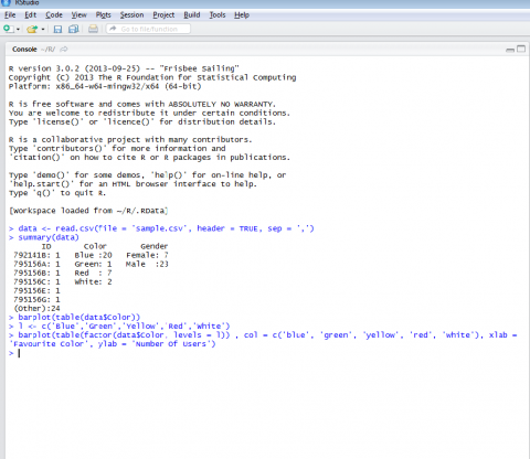
Figure 5-7

Once the graph is labeled, colored, and scaled to the appropriate range, it will look like Figure 5-8 below.

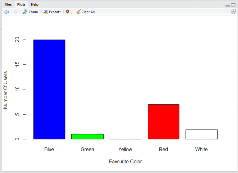
Figure 5-8​