Developing Scatterplots  |  Tutorial Main Menu |  Statistical Analysis Part 2

Section 4: Statistical Analysis

Linear Regressions in R

After importing the dataset Beer, and creating a scatterplot, it is time to code a regression line. Since the data is better skewed with calories as X and alcohol as Y, we will use those variables to code the line. A scatterplot was shown in Figure 4-1 from the following code:

Beer =read.csv("Beer.csv") -- Imported the dataset Beer

attach(Beer)                      -- attached Beer

plot(calories,alcohol)          -- plotted calories and alcohol on the X and Y axis respectively

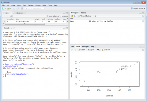
Figure 4-1

After coding the scatterplot, we will now create a trendline through the data using this code:

fit =lm(alcohol~calories, data=Beer)

This defines the linear model as you can see in the workspace

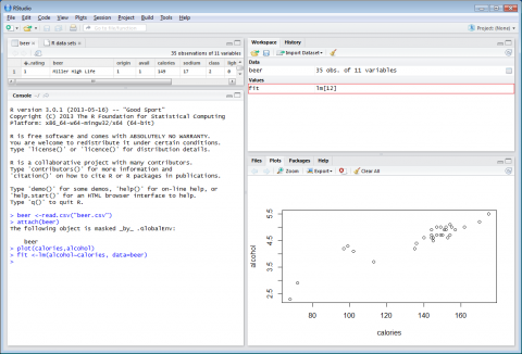
Figure 4-2

Next is the lines function, which places a line through the points as shown in Figure 4-3 below. The $ references the variable to the given data set and fitted formats the line.The code is as follows:  

lines(Beer$calories, fitted(fit), col="orange")

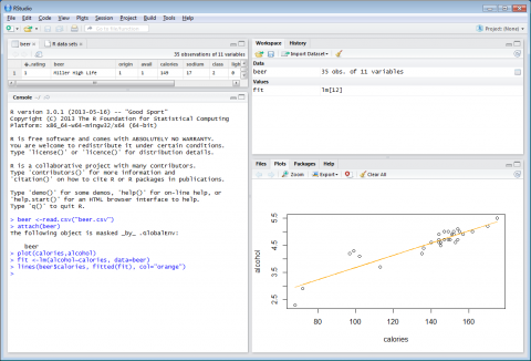
Figure 4-3

You can even use the abline function to place a vertical line of slope(written as v) through the data. The code is as follows:

NOTE: A horizontal line can also be created by using h(for horizontal) rather than v(for vertical).

abline(v=110, col="blue")

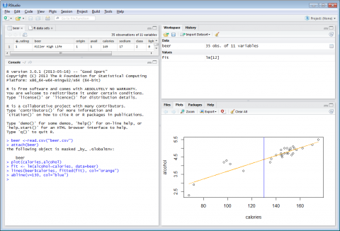
Figure 4-4

Time Series in R

Lets say that each unit of a product represents 1 dollar. We want to see(graphically) how the increase in money corresponds to the passing of years.

A printed time series is displayed in the workspace.

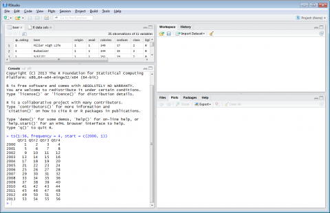
Figure 4-5

Since the variable we would like to view is Money, we will define it in the following code:

money =ts(cumsum(1+round(rnorm(100), 2)), start = c(2000, 7), frequency = 12)

Where the 1 is the x axis multiplied by itself (each # times that digit) 100 represents the max value on the y axis, 2 is the starting value on the y axis, 2000 is the starting year on the x axis, 7 is the number of years and 12 is the frequency.

This will generate a money field in the workspace displaying the time series of [100].

Figure 4-6

Once the time series has been defined you can plot the graph by using the plot function:

plot(money)...or in this case plot(money, col="purple") to change the line color to purple.

Figure 4-7

If you would like a more drastic skew in order to get a better visual of data fluctuations, you may alter the money function so that the data is depicting either a shorter timeframe or a smaller amount of money as shown in Figure 4-8 below.

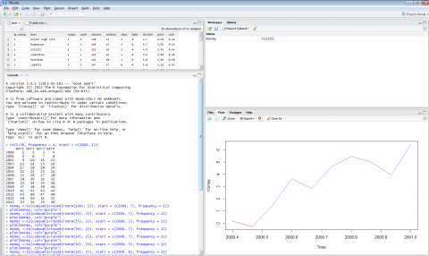
Figure 4-8

Missing Values in R

R identifies unknown numbers(missing values) by the abbreviation NA. In order to demonstrate how R reads data with missing values, we will create two variables: x1 and x2 

Each variable below is known as a Vector

x1 = c(1, 4, 3, NA, 7)                      -- Numeric Vector                                       

x2 = c("A", "B", NA, "NA")             -- Character Vector

Notice that R knew to label each value as Numeric and Character in Figure 4-9 below

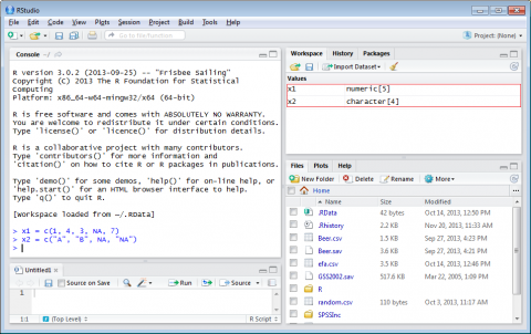
Figure 4-9

To better determine which values are missing in a given vector, we will use the is.na function.The missing values will show up as TRUE whereas the non-missing values will be labeled as FALSE.

For example, to find the missing values of x1 and x2:

x1 = c(1, 4, 3, NA, 7) 

is.na(x1)              FALSE FALSE FALSE TRUE(NA) FALSE

x2 = c("A", "B", NA, "NA") 

is.na(x2)              FALSE FALSE TRUE(NA) FALSE

Other NA functions in R:

na.omit and na.exclude                     Returns the object with observations removed if they contain                                                                 ANY missing values.

na.pass                                              Returns the object unchanged.

na.fail                                                Returns the object ONLY if it contains NO missing values.

The na.omit function and the returned values for the x1 and x2 vectors would show as follows:

x1 = c(1, 4, 3, NA, 7) 

na.omit(x1)        1, 4, 3, and 7 (does NOT return the NA because that is the missing value)

x2 = c("A", "B", NA, "NA") 

na.omit(x2)        A, B, and NA (only one NA is shown because the non-quoted NA resembled the                                                  missing value)

Figure 4-10

We will now use the dataset anscombe(built into R) to display data while setting a few values to NA.

anscombe =within(anscombe, {y1[1:3] =NA})

anscombe...prints the data 

   

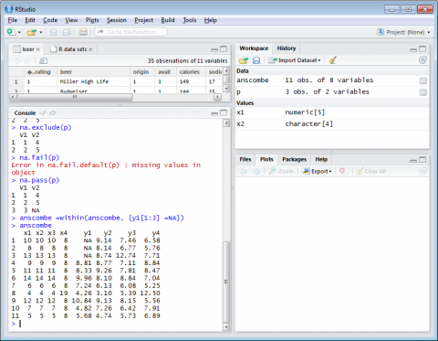
Figure 4-11

We will first define the omissions and exclusions for the missing values within anscombe:

model.omit <- lm(y2 ~ y1, data = anscombe, na.action = na.omit)

model.exclude <- lm(y2 ~ y1, data = anscombe, na.action = na.exclude)

Now we are going to compare missing values on residuals we will use the following code:

resid(model.omit)

resid(model.exclude)

Notice with the model.exclude function it shows the missing values(1, 2, and 3) with NA as as placeholder.